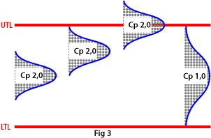
The Cp index describes process capability; it is the number of times the spread of the process fits into the tolerance width. The higher the value of Cp, the better the process.
Example: if Cp = 2.5, the spread of the process fits 2½ times into the tolerance width, while Cp = 1 means that the spread is equal to the tolerance width.
Note that even if the spread is off-centre, it is still the same size (Cp index). The figure takes no account of where the spread is positioned in relation to the upper and lower tolerance limits, but simply expresses the relation ship between the width of the spread and the tolerance width (see Fig. 3).
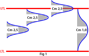
The Cm index describes machine capability; it is the number of times the spread of the machine fits into the tolerance width. The higher the value of Cm, the better the machine.
Example: if Cm = 2.5, the spread fits 2½ times into the tolerance width, while Cm = 1 means that the spread is equal to the tolerance width.
Note that even if the spread is off-centre, it is still the same size (Cm index). The figure takes no account of where the spread is positioned in relation to the upper and lower tolerance limits, but simply expresses the relation ship between the width of the spread and the tolerance width (see Fig. 1).
Cpk (capability process index)
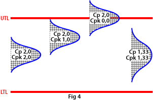
If you also want to study the position of the process in relation to the tolerance limits, you use the Cpk index, which describes the process capability corrected for position. It is not much use having a high Cp index if the process setting is way off centre in relation to the middle of the tolerance range.
A high Cpk index means, then, that you have a good process with a small spread in relation to the tolerance width, and also that it is well centred within that width. If Cpk is equal to Cp, the process is set to produce exactly in the middle of the tolerance range (see Fig. 4).
A normal requirement is that Cpk should be at least 1.33.
Cmk (capability machine index)
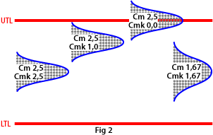
If you also want to study the position of the machine’s capability in relation to the tolerance limits, you use the Cmk index, which describes the capability corrected for position. It is not much use having a high Cm index if the machine setting is way off centre in relation to the middle of the tolerance range.
A high Cmk index means, then, that you have a good machine with a small spread in relation to the tolerance width, and also that it is well centred within that width. If Cmk is equal to Cm, the machine is set to produce exactly in the middle of the tolerance range (see Fig. 2).
A normal requirement is that Cmk should be at least 1.67.
Control limits are an important aspect of statistical process control. They have nothing to do with tolerance limits, because they are designed to call your attention when the process changes its behaviour.
An important principle is that control limits are used along with the mean value on the control graph to control the process, unlike tolerance limits, which are used along with individual measurements to determine whether a given part meets specifications or not.
The function of control limits is to centre the process on the target value, which is usually the same as the middle of the tolerance width, and to show where the limit of a stable process lies. This means, in principle, that you have no reason to react until the control chart signals certain behaviour.
A commonly used control graph is the XR graph, where the position and spread of the process are monitored with the help of sub groups and control limits.
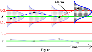
If a point falls outside a control limit on the X graph, the position of the process has changed (see Fig. 16).
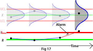
If a point falls outside a control limit on the R graph, the spread of the process has changed (see Fig. 17).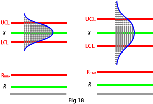
These are the factors that are generally regarded as causing variation in capability measurements:
Centring value for target value
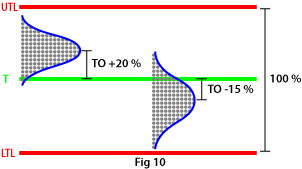
This is the distance from the target value T to the mean value of the machine or process spread (the hump on the normal distribution curve), expressed as a percentage of the tolerance width (see Fig. 10).
There is less talk of centring value for target value nowadays, but the maximum permitted deviation used to be in the region of TO +15%.
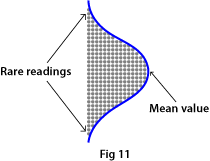
Also called the bell curve because of its shape, this is the pattern in which measurement readings are distributed in most cases as a result of random variations about the mean value (the highest point on the hump, see Fig. 11).
Note that most of the readings are grouped near the hump; the farther out toward the edges, the fewer the readings. In other words it is not very likely that you will find any components at all giving widely deviant readings when making normal spot-check measurements. So it is not enough that the components you happen to measure are all within the tolerances.
It takes measurements of a large number of components to determine the size and shape of the bell curve, and that can be time-consuming. But the standard deviation offers you a shortcut!
Machine capability
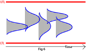
Machine capability is measured in Cm and Cmk; it is a snapshot picture that shows how well a machine is performing right now in relation to the tolerance limits. Figure 6 shows some examples.
Process capability
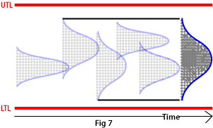
Process capability is a long-term study, measured in Cp and Cpk, that shows how well a process is performing in relation to the tolerance limits while the study is in progress, as well as indicating likely performance in the immediate future.
You could say that process capability is the sum of a index of machine capabilities measured over a period of time (see Fig. 7).
When measuring process capability, you must include everything that affects the process, i.e. all six factors.
| Machine capability | Process capability | |||
Index |
Cm and Cmk | Cp and Cpk | ||
|---|---|---|---|---|
Factors influencing result |
Machine & measurement | All six factors | ||
Stoppages |
Not to be included | Included | ||
Adjustments |
Not to be included | Included | ||
No. of components |
20–50 in succession | 50–250 | ||
Time |
Short | Long |
One standard deviation
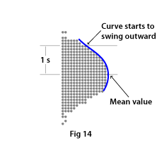
This is a statistical function used to calculate the normal distribution curve, for example. The procedure is that you measure the distance from the mean value (highest point on the hump) to the point where the curve changes direction and starts to swing outward. This distance constitutes one standard deviation (see Fig. 14).
This means that you do not need to measure hundreds of components to find out how much the machine or process is varying. Instead you can calculate the spread using the standard deviation (see below).
Six standard deviations
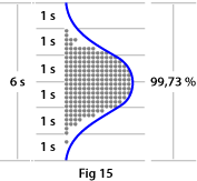
To calculate the normal distribution spread, you simply multiply the standard deviation by 6 to get the total width of the normal distribution curve. If you had gone on making measurements you could have plotted the curve, but now you have calculated it instead (see Fig. 15).
Imagine a shaft fitted in a round hole.
If the diameter of the shaft is on the large side, it leaves less-than-optimum room for lubricant between the shaft and the hole. This results in poorer lubrication, faster wear and shorter lifetime.
A smallish diameter, on the other hand, means greater-than-optimum play. The play tends to increase faster, which also shortens lifetime.
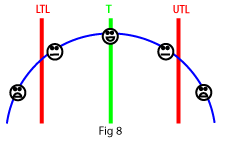
The assembly works best at the target value T, which in this case is in the middle of the tolerance range (see Fig. 8)
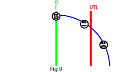
For unilateral properties such as run-out, surface smoothness or mechanical strength, the target value is zero (see Fig. 9).
Statistical process control lets you centre your process on the target value.


How are control limits determined?
The correct way is to let the control limits adapt to the process. That way, a smaller spread in the process gives a narrower control zone, while a greater spread gives a wider control zone (see Fig. 18).
Other ways of determining control limits
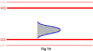
In some cases there may be difficulties about letting the control limits adapt to the process. One such case is where the process uses tools that are not easily adjustable, such as fixed reamers or punches.
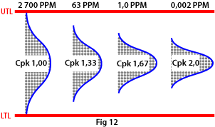
In a quality control context, PPM stands for the number of parts per million (cf. percent) that lie outside the tolerance limits. Cpk 1.00 means that 2 700 PPM (0.27%) of the manufactured parts are out of tolerance, while Cpk 1.33 means that 63 PPM (0.0063%) are rejects.
Note that the PPM index can be drastically improved by a relatively small improvement in the capability index (see Fig. 12).
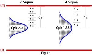
Six Sigma is a philosophy and a mindset for quality improvement used by companies and organisations. The method focuses on minimising waste by minimising variations in processes.
In concrete terms, Six Sigma means that the company's processes maintain six standard deviations from the mean value of the process to the nearest tolerance limit. It follows from this that Cpk 2.0 gives 6 sigma, while for example Cpk 1.33 gives 4 sigma (see Fig. 13).
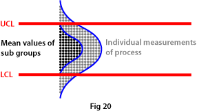
A sub group consists of a number of individual measurements (normally three, four or five) made in sequence from a process. The mean value of these sub- groups, like the process itself, follows a normal distribution curve (see Fig. 20).
Mean values show much less variation compared to individual measurements. This fact, combined with control limits which follow the process in a control graph, means that the machine operator no longer over reacts compared to when adjustment of the process is based on individual measurements. The operator will therefore, as a rule, both measure and adjust the process less often, while at the same time quality will be better.